9 Tuning And Comparing Prediction Models
Evaluating models using the various performance metrics discussed in Chapter 7 gives us a sense of the absolute performance of a model. This can be useful if we have specific criteria that need to be met for a model. For example, we may require a linear regression models to meet a certain RMSE for it to be acceptable. In other situations, we may want to know if there are ways in which we can change the model to improve its performance with respect to a given metric. Depending on the type of prediction model we are using, there can be various ways to make changes. In addition, we need to build upon the approach described in Chapter 7 when there are multiple models whose performance we want to compare.
9.1 The Collection of Models
When building prediction models in practice it is common to consider a collection of possible models and choose the best one from that collection. For the purposes of this chapter the collection of possible models will be defined according to two broad criteria. The first is in terms of the range of possible model classes. Here, we consider a model class as a particular algorithm or approach. We may be interested in comparing the performance of two different model classes in predicting a given outcome. The second criterion for defining a collection of models is the range of tuning parameters associated with a given model class. Not all model classes will have tuning parameters, but most do. For example, with \(k\)-nearest neighbors, the value of \(k\) is the tuning parameter. Different values of \(k\) lead to different models with different performance characteristics.
Often, the simplest approach will be to choose a single model class and then compare models with different tuning parameters within that model class. If this approach leads to a model with satisfactory performance, then that might be all that is needed. However, we may switch to a different model class (and a different set of tuning parameters) if we seek a model with still better performance.
9.2 Model Comparison Workflow
Comparing models within a collection of models introduces a problem that we have not yet encountered because will need to evaluate multiple performance metrics. In Chapter 7 we described a workflow that was valid for evaluating a single prediction model by splitting our dataset into separate training and testing datasets. A key constraint in that scenario was that we can only use the testing dataset once to evaluate the performance of a model. But how can we evaluate multiple models if we can only use the testing dataset once?
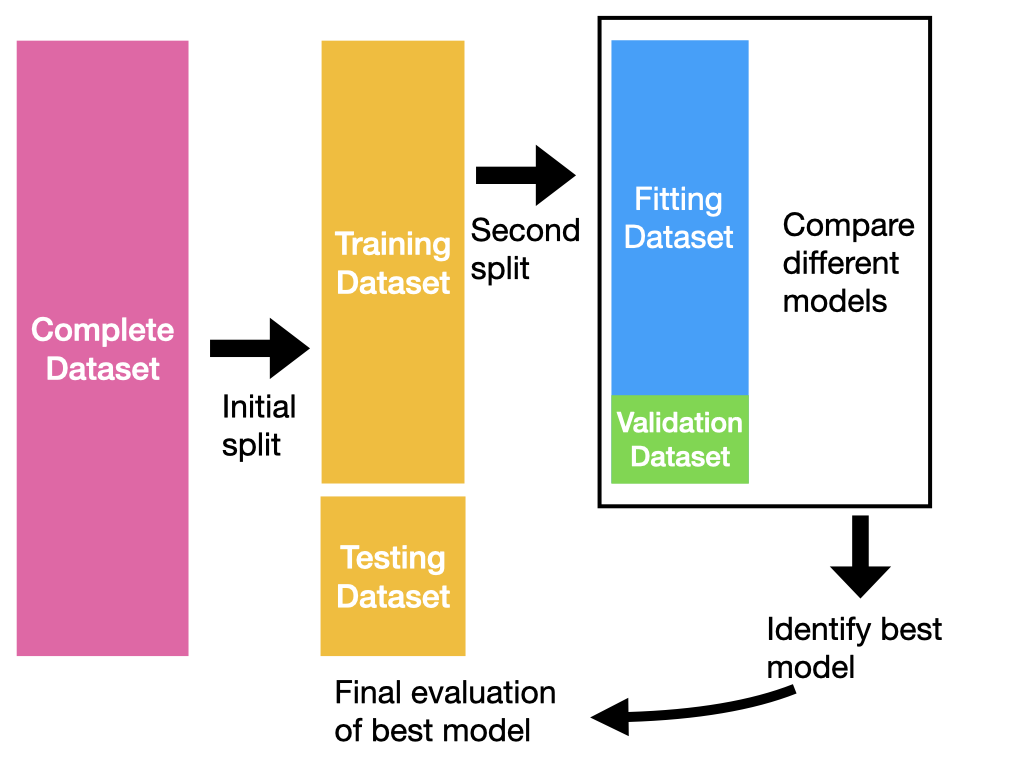
One answer is to split the training dataset again into separate “fitting” and “validation” datasets. The general idea is we can take each of our models/tuning parameter combinations in our collection, fit them all to the fitting dataset, and compute all their performance metrics on the validation dataset. Once we have all the performance metrics computed, we can choose the model with the best metric. Then we can take this best model, fit it to the entire training dataset, and evaluate it on the testing dataset. Here, we do all of our model exploration on the training dataset and only use the testing dataset once we have our final model. A schematic of this general approach is shown in Figure 9.1.
One challenge with this approach is that we are splitting the dataset yet again in order to have independent fitting and validation datasets to do model comparison. Given the reduced size of the dataset at his point, our estimates of model performance metrics may be noisy. One way we can work around possibly noisy estimates of model performance is to estimate the performance on multiple versions of the fitting dataset and average the estimates together. This approach is known as \(v\)-fold cross-validation.
The basic process for \(v\)-fold cross-validation is as follows.
Take the complete dataset and do an initial split into training and testing datasets.
Take the training dataset and divide it into \(v\) “folds” or approximately equal-sized blocks of observations. For \(v\)-fold cross-validation \(v\) is an integer value usually like 5 or 10. Thus for 5-fold cross-validation we would divide the training dataset into 5 equal-sized groups of observations.
Create a fitting dataset by using \(v\)-1 folds of the data and fit a model to this dataset.
Create a validation dataset by using the leftover fold of the data not used for the fitting dataset. Use this validation dataset to compute the performance metric.
Repeat steps 3–4 a total of \(v\) times and estimate \(v\) versions of the performance metric.
Average the \(v\) estimates of the performance metric to obtain the final estimate.
Figure 9.2 shows a depiction of 5-fold cross-validation. For this setup, we would fit and evaluate a model 5 times using each of the different permutations of the 5 folds of the training data. Each time we fit and evaluate a model we get an estimated performance metric \(m_i\) for \(i = 1,\dots,5\). Then we would average the 5 different estimated performance metrics to get \[ M = \frac{1}{5}\sum_{i=1}^5 m_i. \] \(M\) is the final estimate of the performance metric for a given model.
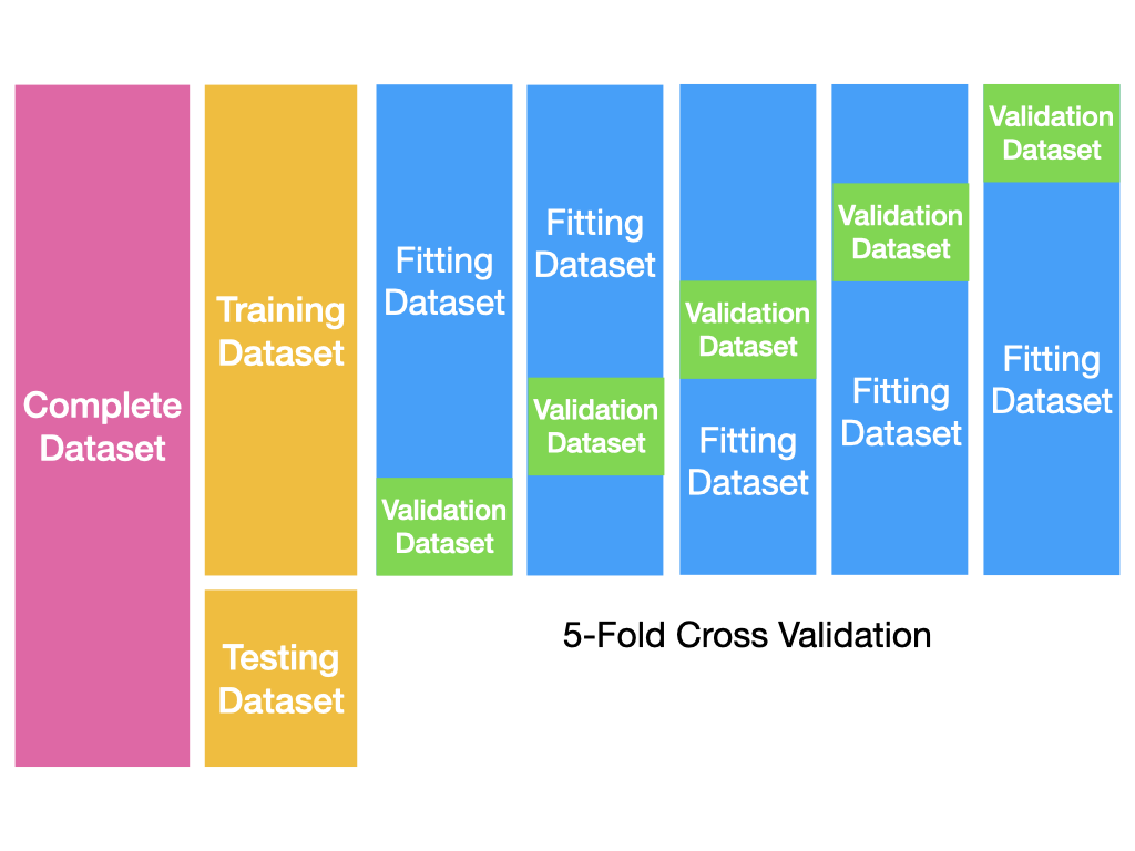
We can repeat this entire process for a different model to get a different performance estimate. The averaging of the individual performance metric estimates \(m_i\) smooths out the variation across the different possible configurations of the dataset.
9.2.1 Example: Predicting Miles Per Gallon
To illustrate the process of model comparison we will use a small dataset to make it simpler to visualize what is happening with the data and the models. We will use the mtcars dataset from the tidyverse package for this illustration. This dataset contains information about the mile per gallon of gasoline achieved on 32 different cars.
The first thing we will do is randomly split the dataset into a training and testing dataset using an 80/20 ratio. This means that \(0.8 \times 32 \approx 25\) cars will be in the training dataset and \(32-25=7\) cars will be in the testing dataset. For this random split, the training dataset is shown in Table 9.1 below.
mtcars data.
| mpg | cyl | hp | wt | |
|---|---|---|---|---|
| Cadillac Fleetwood | 10.4 | 8 | 205 | 5.2 |
| AMC Javelin | 15.2 | 8 | 150 | 3.4 |
| Datsun 710 | 22.8 | 4 | 93 | 2.3 |
| Merc 450SE | 16.4 | 8 | 180 | 4.1 |
| Merc 450SL | 17.3 | 8 | 180 | 3.7 |
| Fiat 128 | 32.4 | 4 | 66 | 2.2 |
| Toyota Corona | 21.5 | 4 | 97 | 2.5 |
| Merc 230 | 22.8 | 4 | 95 | 3.1 |
| Merc 280C | 17.8 | 6 | 123 | 3.4 |
| Merc 240D | 24.4 | 4 | 62 | 3.2 |
| Ford Pantera L | 15.8 | 8 | 264 | 3.2 |
| Volvo 142E | 21.4 | 4 | 109 | 2.8 |
| Dodge Challenger | 15.5 | 8 | 150 | 3.5 |
| Camaro Z28 | 13.3 | 8 | 245 | 3.8 |
| Mazda RX4 | 21.0 | 6 | 110 | 2.6 |
| Pontiac Firebird | 19.2 | 8 | 175 | 3.8 |
| Merc 450SLC | 15.2 | 8 | 180 | 3.8 |
| Lotus Europa | 30.4 | 4 | 113 | 1.5 |
| Ferrari Dino | 19.7 | 6 | 175 | 2.8 |
| Porsche 914-2 | 26.0 | 4 | 91 | 2.1 |
| Lincoln Continental | 10.4 | 8 | 215 | 5.4 |
| Honda Civic | 30.4 | 4 | 52 | 1.6 |
| Fiat X1-9 | 27.3 | 4 | 66 | 1.9 |
| Hornet 4 Drive | 21.4 | 6 | 110 | 3.2 |
| Mazda RX4 Wag | 21.0 | 6 | 110 | 2.9 |
In general, we will not want to look at the testing dataset and will rather set it aside until we have selected our final model. But for the purposes of this demonstration, we can see the testing dataset in Table 9.2.
mtcars data.
| mpg | cyl | hp | wt | |
|---|---|---|---|---|
| Hornet Sportabout | 18.7 | 8 | 175 | 3.4 |
| Valiant | 18.1 | 6 | 105 | 3.5 |
| Duster 360 | 14.3 | 8 | 245 | 3.6 |
| Merc 280 | 19.2 | 6 | 123 | 3.4 |
| Chrysler Imperial | 14.7 | 8 | 230 | 5.3 |
| Toyota Corolla | 33.9 | 4 | 65 | 1.8 |
| Maserati Bora | 15.0 | 8 | 335 | 3.6 |
We will not use the testing dataset until we have selected our final model.
The first model we will look at will predict the mpg variable using the hp or horsepower variable, wt (weight), cyl (number of cylinders) variables. We will use a \(k\)-nearest neighbors regression here as our prediction model and we want to estimate the root mean squared error (RMSE) and the \(R^2\) value for this model. Initially, we will set the value of \(k\) to be 4.
We will now proceed with a 5-fold cross-validation process to estimate the performance metrics. This will involve splitting the training dataset into a fitting and validation dataset. Using an 80/20 ratio again, we will take the 25 observations in the training dataset and randomly split them into 20 observations for the fitting dataset (\(20 = 0.8\times 25\)) and 5 observations for the validation dataset. In the first “fold” of the 5-fold cross-validation, our procedure randomly selected observations 2, 3, 12, 18, 21 for the validation dataset and the remaining 20 for the fitting dataset. Using this split, we fit the \(k\)-nearest neighbors model to the 20 observations in the fitting dataset and compute the RMSE and the \(R^2\) using the 5 observations in the validation dataset. Doing so gives us an RMSE of 2.24 miles per gallon and an \(R^2\) of 0.95. If we continue for four more iterations using the four remaining folds of the data, we get the following RMSE and \(R^2\) values for each of the folds (Table 9.3).
| Fold | RMSE | \(R^2\) |
|---|---|---|
| 1 | 2.24 | 0.95 |
| 2 | 2.38 | 0.70 |
| 3 | 1.74 | 0.88 |
| 4 | 1.66 | 0.93 |
| 5 | 3.46 | 0.90 |
It is clear from Table 9.3 that there is some variation in both the RMSE and \(R^2\) values across the different folds. To obtain the final estimates we will average the RMSE and \(R^2\) values across the folds to obtain our final values. Table 9.4 shows the final average values along with a standard error measure.
| Metric | Mean | Std. Error |
|---|---|---|
| RMSE | 2.30 | 0.32 |
| $R^2$ | 0.87 | 0.04 |
What happens if we change the value of \(k\) in the \(k\)-nearest neighbors method? Would we do any better? We can try using a value \(k=9\) and see how the method performs. Using the same cross-validation procedure, we can obtain an estimate of the RMSE and \(R^2\) when \(k=9\). Those results are shown in Table 9.5.
| Metric | Mean | Std. Error |
|---|---|---|
| RMSE | 2.83 | 0.32 |
| \(R^2\) | 0.87 | 0.04 |
We can see that with \(k=9\) the RMSE appears to go up and the \(R^2\) appears to be unchanged, relative to the model with \(k=4\). Based on RMSE, the performance is worse when \(k=9\); based on \(R^2\) is is about the same, suggesting we might prefer the \(k=4\) version of the model.
Finally, using the \(k=4\) version of \(k\)-nearest neighbors, we can fit the model to the entire training dataset and evaluate the RMSE and \(R^2\) on the 7 observations in the testing dataset (which we have yet to use at this point). The final results are shown in Table 9.6.
| Metric | Estimate |
|---|---|
| RMSE | 2.45 |
| \(R^2\) | 0.89 |
In Table 9.6 we can see that the final RMSE is a little be higher in the testing dataset than it was in the training dataset. This likely reflects regular statistical variation as we are using different data points here for the evaluation. With larger datasets this kind of variation is likely to go down as we are able to obtain more stable estimates of the performance metrics.
9.3 Optimizing Tuning Parameters
One feature of the example in the previous section was that we compared two versions of the \(k\)-nearest neighbor models—one with \(k=4\) and one with \(k=9\). In that case, the version with \(k=4\) appeared to perform better, but it is possible that another version of \(k\) would have worked even better. With most prediction models, it’s useful to check a range of possible tuning parameter values in order to makes sure that we have found the value that produces the best prediction. Other methods also have more than a single tuning parameter, and so it might be necessary to try different combinations of multiple tuning parameters to find the optimal set.
Continuing the example from the previous section where we were predicting miles per gallon, we can try multiple values of \(k\) for the \(k\)-nearest neighbors algorithm. Here, we will try values between 1 and 11. For each of these values of \(k\) we will run a 5-fold cross-validation in order to obtain an estimate of the RMSE and the \(R^2\). Figure 9.3 shows the RMSE values for each value of \(k\) based on a 5-fold cross-validation on the training dataset.
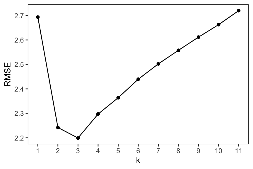
We can see clearly that the minimum RMSE value on the plot appears to occur at \(k=3\). This suggests that while in the previous section we observed that \(k=4\) was a better model than using \(k=9\), there was in fact a still better model that we could have chosen with \(k=3\).
Figure 9.4 shows the same kind of plot but with the \(R^2\) metric instead.
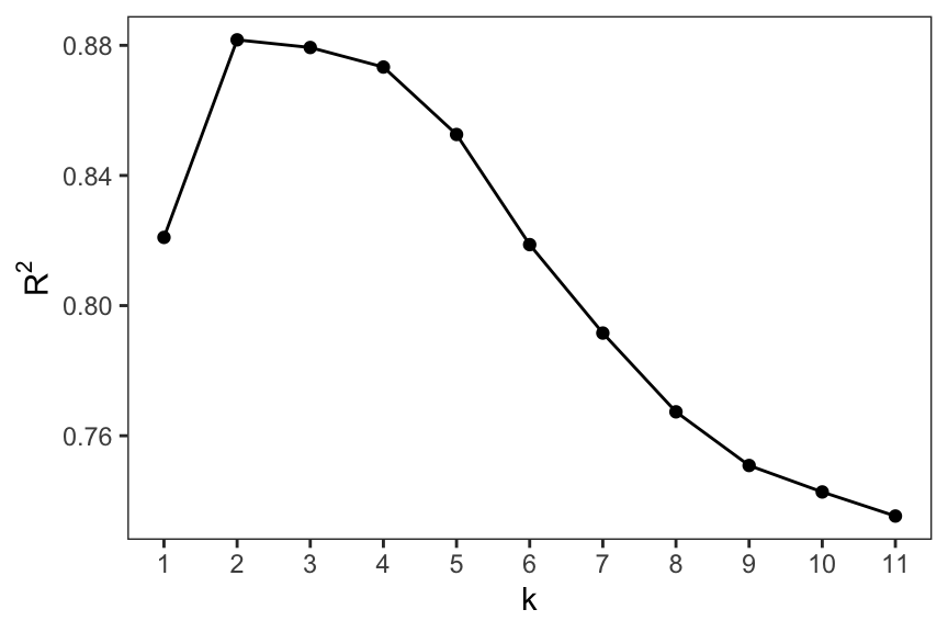
We can see here that the maximum \(R^2\) value occurs with a value of \(k=2\). In general, it’s not necessarily true that different metrics will identify the same optimal tuning parameter, as we have seen here. However, in Figure 9.4, it seems that the \(R^2\) for \(k=3\) is quite close to the \(R^2\) value for \(k=2\). So if we were going to choose a best model, we might choose \(k=3\) given that its \(R^2\) values nearly the same as the optimal value and there is a distinctly better RMSE value. Otherwise, if there is disagreement between different metrics, we might choose the optimal \(k\) value based on which metric is more important in the context of the application.
9.4 Example: Classifying Clothes
In this case study we will use the Fashion MNIST dataset which contains images of different kinds of articles of clothing. The images are grayscale and are 28 by 28 pixels in dimension. The dataset contains 10 different types of clothing but we will focus on just two: T-shirts and shirts. A sample of a few columns and rows of the dataset are shown in Table 9.7.
| label | pixel541 | pixel710 | pixel728 | pixel321 | pixel507 |
|---|---|---|---|---|---|
| 0 | 191 | 189 | 0 | 129 | 0 |
| 6 | 180 | 163 | 0 | 207 | 0 |
| 0 | 131 | 162 | 0 | 169 | 0 |
| 0 | 220 | 213 | 0 | 217 | 0 |
| 0 | 83 | 0 | 0 | 255 | 0 |
Each row of the table represents a single image article of clothing. The first column represents the identifier of whether the piece of clothing is a T-shirt (label = 0) or a shirt (label = 6). The remaining columns are the values of the individual pixels in the image (0 represents white and 255 represents black). There are a total of \(28\times 28=784\) pixels in each image, with each pixel representing a column in the dataset. A representative image of each clothing class is shown in Figure 9.5.
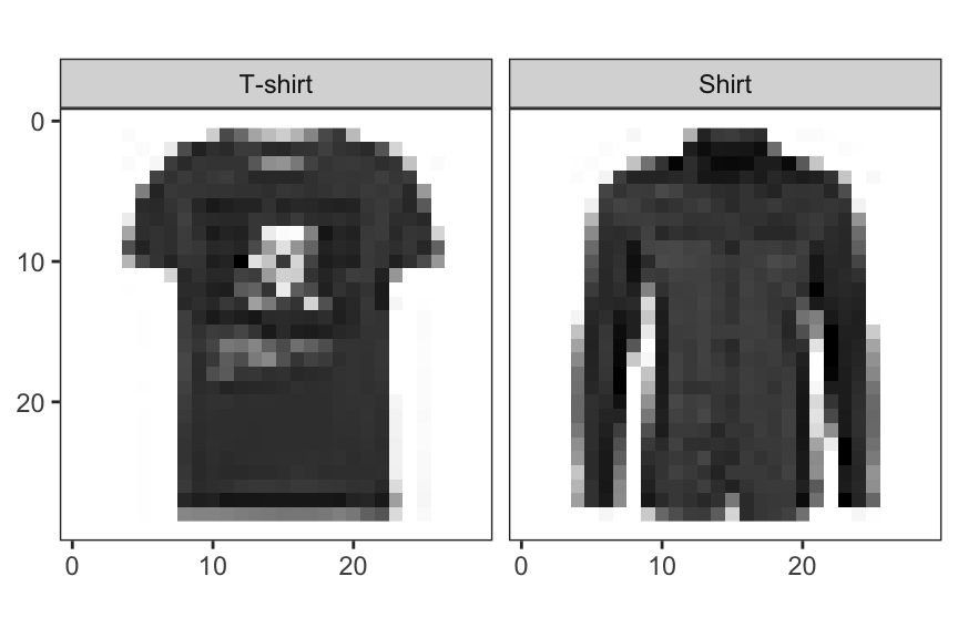
The goal of this prediction case study is to build a prediction model that can classify each image into a T-shirt or a shirt based on the image pixel values. For this example we will use the random forest algorithm described in Chapter 8. The random forest algorithm has a tuning parameter named \(m\) that represents the number of variables to use when determining a split point when it is growing a decision tree. The performance of the algorithm can vary with the value of \(m\) so we will assess the accuracy of the predictions as the value of \(m\) changes.
We first split the data into training and testing datasets using an 80/20 split proportion. We then use values of \(m\) ranging from 1 to 5 and compute the accuracy of the predictions using 10-fold cross-validation on the training dataset. The esimated accuracy as a function of \(m\) is shown in Figure 9.6.
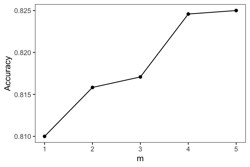
We can see from Figure 9.6 that even for an \(m\) value of 1 the accuracy is already around 0.8. However, for larger values of \(m\) the accuracy appears to go up, with an accuracy of greater than 0.82. In Figure 9.6, we see that the maximum accuracy value occurs when \(m = 5\), which is at the boundary of our range of \(m\) values that we explored. Therefore, it is possible that there is a value of \(m\) that produces an even higher accuracy, but we don’t know that because we haven’t explored beyond 5.
When we see that an optimal tuning parameter occurs on the boundary of our range, it’s usually a good idea to expand the range a little further to see if there are in fact better values of that tuning parameters. Here, we will expand the range to look at \(m\) values from 1 to 10. The results are shown in Figure 9.7.
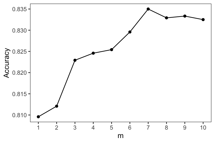
Figure 9.7 shows that an \(m\) value of 7 produces an accuracy of about 0.835, which looks like a local maximum. Using \(m = 8\) produces an accuracy that is slightly lower. From Figure 9.7, it would seem that \(m=7\) is the optimal value.
Overall, the range of accuracy values in Figure 9.7 is relatively small, ranging from 0.810 to 0.835. However, in some applications, it may be important to squeeze out an addition few percentage points of accuracy by tuning the model a little. Choosing an \(m\) of 7 over an \(m\) of 1 would give about 2 extra percentage points of accuracy.
In the previous section, Figure 9.3 seemed to clearly indicate an optimal value of the tuning parameter \(k\) and it did not seem like there would be a better value outside the range of the plot. In Figure 9.7, we appear to achieve a local maximum for \(m\) of 7. However, even though \(m\) of 10 produces a lower accuracy, there is no guarantee that values of \(m\) larger than 10 will produce even lower accuracies. It could be that larger values will increase accuracy beyond \(m\) of 11. While it can be very time-consuming, particularly if the dataset is large, if optimizing the accuracy is important, it can be a good idea to expand the range of tuning parameters to make sure that you have in fact achieved the maximum accuracy. Another possibility is that the accuracy levels off after a certain value of \(m\). Either way, expanding the range of possible values may be an important part of tuning the model.
Finally, we can take our best model with and re-fit the model to the entire training dataset. Then we can use the testing dataset (which we have not used yet) to compute the final accuracy of the model. Here, we achieve an accuracy of 0.81 on the testing dataset, which is slightly lower than what we estimated in the cross-validation.
9.5 Further Notes On Tuning
So far we have shown how the model tuning process works for a single tuning parameter. In practice, most models have multiple tuning parameters that will need to optimized simultaneously. Even the random forest algorithm that we used in the previous section has three tuning parameters—we simply ignored the other two for the example. However, it would be prudent to attempt to optimize over the other two parameters if time permits. Doing so would require searching over a grid of possibilities. For example, we might want to try \(m\) values ranging from 8 to 12 and the number of trees equal to 500 and 1000. Then the grid of possibilities would look as follows.
| m | ntree |
|---|---|
| 8 | 500 |
| 10 | 500 |
| 12 | 500 |
| 8 | 1000 |
| 10 | 1000 |
| 12 | 1000 |
As with any estimation process, there is a certain amount of uncertainty that must be accepted when optimizing a model over its tuning parameters. If the training dataset is quite large, then estimates of performance will generally be stable across a range of tuning parameters and the optimal model, however defined, will likely be clear. However, with smaller datasets, or perhaps with weaker models, there might appear to be multiple combinations of parameters that produce equivalent models. This is often a fact of the tuning process, where it may not be clear which model is best. In a situation where multiple tuning parameters produce similar performance, one may end up choosing the tuning parameters based on other criteria. For example, if there is a combination of tuning parameters that is faster to train or make predictions and produces reasonable performance, one may choose that combination on this basis.
One method of tuning that we have not discussed involves adding or removing specific predictors or features. In this chapter we have focused primarily on optimizing models using by varying the available tuning parameters for each model. However, sometimes performance can be improved by changing the predictors that are being used. In particular, for linear regression or logistic regression, changing the predictors in the model is essentially the only way to modify the prediction performance of the model (there are no external tuning parameters).
The reason we have not discussed the adding/removing of predictors here is that there is a separate methodology involved with identifying predictors for inclusion into a model and we will discuss that briefly in Chapter 13. Additionally, with flexible models like random forests, a reasonable strategy is to include as many predictors as are available and let the algorithm sort out which predictors are important for predicting the outcome. Flexible models like random forests are designed to effectively “remove” or downweight predictors that are not contributing to predicting performance. That said, it is not always a good idea to simply dump all predictors into a model and see how it performs. With some approaches, having too many predictors in a model will hurt performance.
9.6 Summary
Flexible prediction models often have tuning parameters that can affect how well they perform. Identifying the optimal combination of tuning parameters is usually a key step in any prediction modeling workflow. Comparing models with different tuning model specifications require splitting the training data into separate fitting and validation datasets and computing performance metrics using \(v\)-fold cross-validation. There may be many different combinations of tuning parameters to evaluate using \(v\)-fold cross-validation so this can be a time-consuming process.
Identifying the optimal set of tuning parameters will depend on the range of parameters that are checked. In some cases the best tuning parameter values will be on the boundary of the range that was checked. In those cases, it’s usually a good idea to expand the search space of tuning parameters so that we can be sure that there is not an even better tuning parameter value out there that we haven’t checked. Typically, we want to search the parameters space until we identify a local mode.