7 Evaluating Models
With a linear regression model the predicted outcome for a given unit is the result of plugging in the predictor values into the fitted model, multiplying the estimated coefficients and summing the result. The predicted outcome is \[ \hat{y}=\hat{\beta}_0+\hat{\beta}_1x_1+\cdots+\hat{\beta}_px_p. \] What we do not know, in general, is how close this predicted outcome \(\hat{y}\) is to the true outcome \(y\). Ideally, we would like for our predictions to be close to the true values. In this chapter, we will walk through some of the considerations that are made when defining a “good” prediction model.
When we build a prediction model, we want to be able to say that we are building the model in a manner that will result in good predictions on future data for which we have not yet observed the outcome. But the problem is that we have not yet observed this future data, so how can we know how the model will perform? A key task in building prediction models it so develop some sense of the error that a model will make on future observations while using the data we have at hand.
7.1 The Bias-Variance Tradeoff
Two key model characteristics that will play into our considerations here are
Bias: This is the systematic difference between what the model generally predicts and what we observe. If a model has a bias of zero (i.e. it is “unbiased”), then on average, its predictions will not systematically be greater or less than the observed outcomes.
Variance: This is the variability of the model itself under different training samples. In most situations, we can think of the training data for a model as a random sample from a much larger population. If the model produces very different predictions depending on which random sample we happen to choose, then the model shows high variance. If the model does not vary very much in its predictions when trained under different random samples, then the model exhibits low variance.
From the descriptions of bias and variance, it would see that we would want our models to have both low bias and low variance. This is true, however it turns out that these two features fight against each other, and therefore it can be difficult to minimize both at the same time.
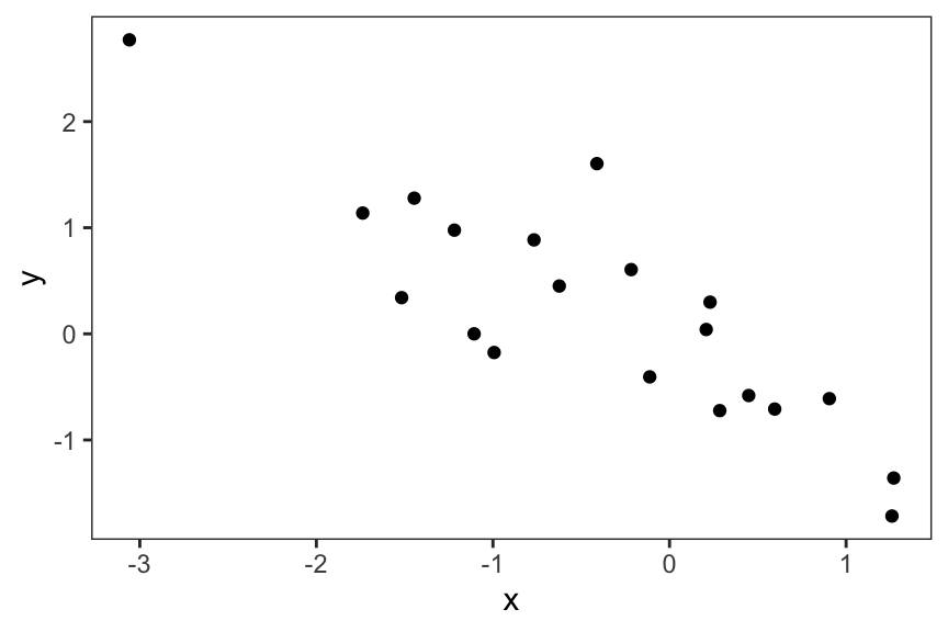
We will use a simple example with a small dataset to illustrate some ideas about bias and variance. Consider the data in Figure 7.1 below and how we might develop a prediction model to prediction the outcomes of future observations.
From the plot, it would appear that the outcome y has a decreasing relationship with the predictor x. At first glance, it would appear that x has some ability to predict the values of y.
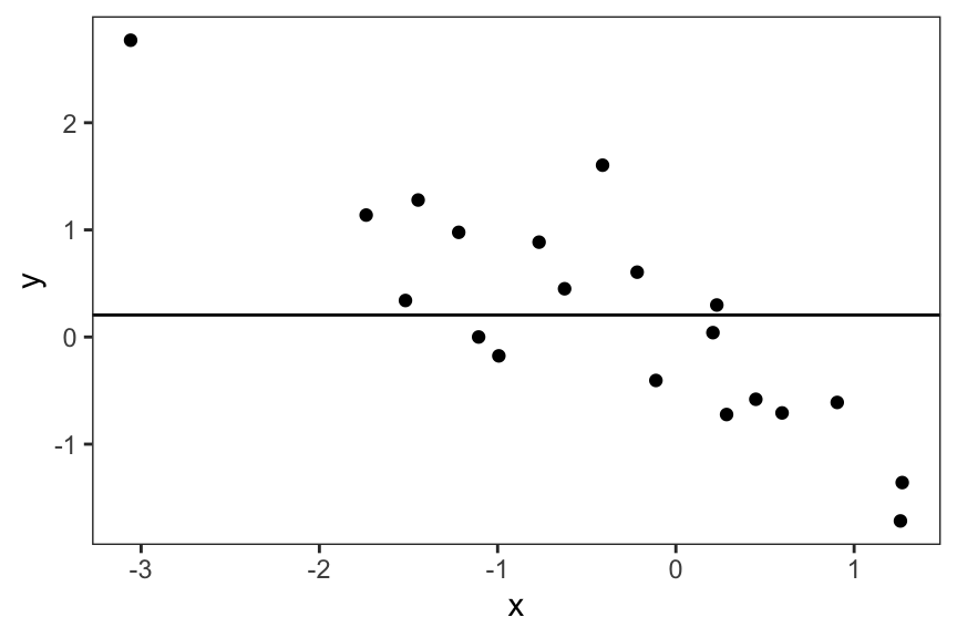
The simplest model that we could employ would be one that uses no predictor information at all. This model would simply use the mean of y as a prediction for any value of x. We have plotted the model below in Figure 7.2. In this model, the predicted value is always 0.21. This is no doubt a silly “model”, but it is one nonetheless.
y.
This model’s predictions are reasonably close to the data for some of the data points, but it systematically underestimates the data when x is less than -1 and systematically overestimates the data when x is greater than 0. This observation suggests that the model is biased in those areas of the domain of x. It’s not hard to imagine that if we drew another sample of data just like this dataset, this constant mean model would exhibit the same biases. In fact, we can simulate a second dataset and see how the model looks on this new dataset relative to the original dataset.
Figure Figure 7.3 shows a second simulated sample along with the mean. In the second dataset, the prediction from the model is always -0.38. We can see from the new sample the constant mean model shows the same types of biases for roughly the same regions of the domain of x.
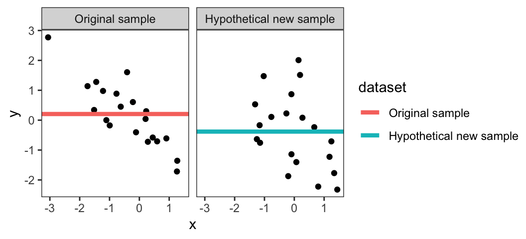
Although this constant mean model seems to exhibit significant biases on the training dataset, one advantage of this model is that its predictions are relatively stable from sample to sample. If we were to draw a new sample, the mean would change a little (as we saw with the second sample), but in general the predictions would remain similar. Therefore, there would be no concern that a model trained with a slightly different sample would make dramatically different predictions for a given value of x.
This is the bias-variance trade-off at work. Models like the constant mean model that have high bias tend to have low variance. Similarly, models with low bias tend to have high variance. In general, it is difficult to find a model that minimizes both bias and variance well.
The plot below in Figure 7.4 shows a different kind of model. Here, we “connect the dots” of the training data to produce a prediction model that actually has zero bias on the training data.
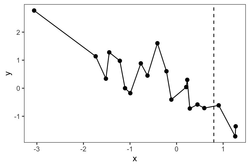
The vertical dashed line in Figure 7.4 represents a value of x for which we want to make a prediction. Because we have no data points at that specific value of x, we will use the solid black interpolation line as our predicted value. Here, the predicted value is approximately -0.6.
What happens if we sample a new dataset and fit this same “connect-the-dots” model to the new dataset? Figure 7.5 shows the original sample and the new sample along with their respective “model fits”. We can see that with the new sample, the model is just as noisy as the original connect-the-dots model.
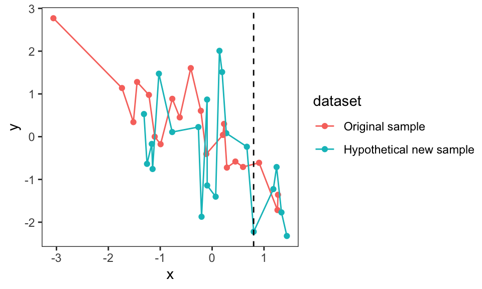
For the predicted value at the x value indicated by the dashed line, we see that in the new sample, our model predicts a value of approximately -2.2. This is quite a bit different from the prediction that we got from the model fitted to the first sample, which was about -0.6. In fact, if we draw a vertical line anywhere along the x-axis, we can see that the predictions from the first sample can be very different from the predictions in the second sample.
We have purposely taken two extreme examples of the kinds of “models” you might fit the data. The constant mean model is an example of a model with high bias but low variance. Asymptotically, if the sample size were to get bigger and bigger, the variability of this model would eventually go to zero. However, the bias of the model would generally not go to zero with larger sample sizes. The connect-the-dots model is example of a model with high variance but low bias. For any given training dataset, the model is designed to have zero bias on the training dataset. However, the predictions that it makes are highly variable, and even if we were to collect more data and increase our training dataset size, the variability of this model would not go down. In particular, the variability of this model is equal to the variability of the data themselves, and so the model does not gain stability with larger sample sizes.
Finally, let’s take a look at what happens if we fit a linear regression model to the data from the first sample and the new sample. Figure 7.6 below shows the linear model fits for both datasets.
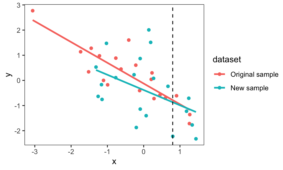
While the linear regression line is different for both datasets, they are qualitatively similar. Neither line shows significant biases in any particular range of the x values. Furthermore, the predicted values from the regression lines at the x value indicated by the vertical dashed line are relatively close. In this case, the linear regression model appears to demonstrate a reasonable balance between having any systematic biases and having significant variability from one sample to the next.
We note that the data for the examples here were simulated so we knew what the true model was, which in this case was a linear regression model. This is why the linear regression fit looks good in these datasets. In general, we will not know the data-generating process and so the linear regression model may not perform so well in all cases.
7.2 Performance Metrics for Regression Models
In the previous section we looked at model predictions at specific values of our predictor variable. However, when evaluating a model, we want something that will evaluate the model’s performance more generally, so that we have a sense of how it might perform at many different predictor values. In this section we will introduce some of these global metrics that allow us to evaluate regression models. In the next section we will cover performance metrics for classification models.
7.2.1 Root Mean Squared Error
The root mean squared error, or RMSE, of a model is a summary of the difference between the observed true value of an outcome and predicted outcome from the model. To define it we need a little notation. Suppose we have a dataset were we observe \(n\) data points, where \(y_1,\dots,y_n\) represent the observed outcome and \(\mathbf{x}_1,\dots,\mathbf{x}_n\) represent the predictor variables. Now suppose we have a model (like a linear regression model) that is represented by the function \(f\) and we can make predictions for any value of \(\mathbf{x}_i\) by plugging it into \(f\) to get \(\hat{y}_i =f(\mathbf{x}_i)\). So \(\hat{y}_i\) is the predicted value for observation \(i\) based on predictor \(\mathbf{x}_i\). Then the RMSE for the model \(f\) is defined as
\[ \text{RMSE} = \sqrt{\frac{1}{n}\sum_{i=1}^n (y_i - \hat{y}_i)^2} \] The RMSE is the square root of the average squared difference between a model’s predicted value and the observed outcome. Importantly, the RMSE has units and the units of the RMSE are the same as the units of \(y_i\). One way that we can interpret the RMSE is that on average, the model is off from the true value by an amount equal to the RMSE. Models with RMSEs that are smaller demonstrate better performance.
What is a good value of the RMSE? In general, we cannot say because the answer will depend on the nature of the data and the problem we are trying to solve. Because the RMSE has units, we can only really interpret it in the context of the specific dataset and problem. Some problems may allow for typical deviations from the truth to be quite wide while other problems may require very small deviations. When considering a specific RMSE value, usually we can only evaluate it when talking with collaborators or others who are knowledgeable of the problem and the data. Often, we are comparing RMSE values between different models (see Chapter 9) and in those cases, we only need to evaluate which model has a smaller RMSE.
7.2.2 \(R^2\) (R-squared)
An alternative performance metric for regression models is the \(R^2\) (or “R-squared”) value. This value measures the proportion of variation in the distribution of the outcome that is “explained” by a prediction model (usually it is stated as a percentage). If a prediction model is good, so that the predictors in the model carry a lot of information about the outcome, then we should be able to use the model to explain why there is variation in the outcome. No model will be able to perfectly predict the outcome, so there may be some residual variation left over, even when using the model. But a good model will minimize that residual random variation.
The \(R^2\) metric is defined as
\[ R^2 = 1-\frac{\sum_{i=1}^n(y_i-\hat{y}_i)^2}{\sum_{i=1}^n (y_i-\bar{y})^2} \] In general, \(R^2\) will be a number between 0 and 1, where 0 represents a model that explains no variation in the outcome and 1 represents a model that explains all of the variation in the outcome.
The \(R^2\) formula is written as 1 minus a fraction. In the denominator of that fraction is the sum of squared deviations between each of the \(y_i\) values and the overall mean of the \(y_i\) values, \(\bar{y}\). This denominator therefore represents the overall or “total” variation in the outcome data \(y_i\). If we multiplied the denominator by \(\frac{1}{n-1}\) we would have the sample variance of the \(y_i\)s. In the numerator of the fraction we have the sum of squared deviations between the observed outcomes \(y_i\) and the model predicted values \(\hat{y}_i\). The numerator therefore represents the overall error of the model, or the total residual variation from the model. If we multiplied the numerator by \(\frac{1}{n}\) we would have the square of the root mean squared error (or just the mean squared error).
From the formula, we can see that if \(R^2=0\), then we have that the overall error of the model (the numerator) is equal to the total variation in the outcome data (the denominator). In other words, the model has a total residual variation that is equal to the total variation. In general, this is the sign of a poor model because it suggests that our uncertainty about the outcome is the same after using the model as it was before using the model. If \(R^2=1\), then that means that the total residual variation is 0, or the overall error of the model is 0. If the model perfectly predicts the outcome, then that would suggest that it can explain all of the variation in the outcome.
7.3 Performance Metrics for Classification Models
In the previous chapter, we noted that logistic regression models produce a predicted probability of the outcome \(Y\) taking a value of 1, i.e. \(\mathbb{P}(Y=1)\). In order to make a classification, we must determine a cutoff value for the predicted probability so that we determine which observations are classified 1s and which are 0s. Some algorithms other than logistic regression are designed to produce discrete classifications as opposed to continuous probabilities (as we will see in later chapters). Nevertheless, when we evaluate a classification model, the output we will use are the discrete classifications that are generated from the model. For now, we will focus on binary classification as that is the most common scenario.
The basic setup for evaluating a classification model involves having two sets of output:
The true outcome classification: This is a vector of the true class values for each observation;
The predicted outcome classification: This is the vector of predicted discrete classifications, possibly obtained after dichotomizing the model output using a cutoff value.
As an example, these outputs might look like the hypothetical results in Table 7.1. The column labeled “True Class” shows the vector of true class values for each observation/row and the column labeled “Predicted Class” shows the vector of predicted classifications from the hypothetical model.
| True Class | Predicted Class |
|---|---|
| 1 | 0 |
| 1 | 0 |
| 0 | 1 |
| 1 | 1 |
| 1 | 1 |
| 0 | 1 |
| 0 | 1 |
| 1 | 1 |
| 1 | 1 |
| 1 | 0 |
From Table 7.1 we can see that in each row of the table, we can characterize the true class and the predicted class in three possible ways:
The true class and the predicted class are the same, either both are 1 or both are 0 (this is a correct classification by the model). When both are 1 this is sometimes referred to as a true positive from the model and when both are 0 this is sometimes referred to as a true negative from the model;
The true class is 0 and the predicted class is 1; this is a false positive from the model;
The true class is 1 and the predicted class is 0; this is a false negative from the model.
Performance metrics for classification models generally involve looking at different ways to compare the true classes to the predicted classes. Determining which performance metric is ideal for a given problem will usually depend on the specifics of a problem. Some problems may favor minimizing the number of false positives, while others may want to minimize false negatives. For example, in a medical diagnosis setting where an algorithm is used to diagnose the presence of a disease, we may want to minimize false negatives because a false negative results in a patient walking away without knowing that they have the disease.
While there are many different classification metrics available, we will focus on just a few of them here. They are shown in Table 7.2.
| Metric | Description |
|---|---|
| Accuracy | Proportion of all observations that are predicted correctly |
| Sensitivity | Proportion of true 1s that are predicted as 1s |
| Specificity | Proportion of true 0s that are predicted as 0s |
| False Positive Rate | Proportion of predicted 1s that are actually 0s |
| Positive Predictive Value | Proportion of predicted 1s that are actually 1s |
The calculation of each of these metrics is perhaps best shown with a small example. Suppose we have a prediction model (like a logistic regression) that classifies observations into two classes (0 and 1). We can make a cross-tabulation of the predicted classes and the true classes in the dataset. Such a cross-tabulation is shown in Table 7.3 and is often referred to as a confusion matrix.
| True 0 | True 1 | Sum | |
|---|---|---|---|
| Predicted 0 | 318 | 142 | 460 |
| Predicted 1 | 39 | 70 | 109 |
| Sum | 357 | 212 | 569 |
In this table, the lower right corner shows the total number of observations in the dataset, which is 569 here. The bottom of the column labeled “True 0” shows that there are 357 true 0s in the dataset and the bottom of the “True 1” column shows that there are 212 true 1s in the dataset. The right side of the “Predicted 0” row shows that 460 observations were predicted to be a 0; the “Predicted 1” row shows that 109 observations were predicted to be a 1.
Each of the performance metrics in Table 7.2 is a proportion, which means that each metric has a numerator and a denominator. The metrics differ based on what they use as their respective numerators and denominators. Table 7.4 shows how each of the classification metrics are calculated from the data in Table 7.3.
| Metric | Denominator | Numerator | Calculation | Value |
|---|---|---|---|---|
| Accuracy | Total Observations | Predicted 0 & True 0 + Predicted 1 & True 1 | (318+70)/569 | 0.68 |
| Sensitivity | Sum of True 1 | Predicted 1 & True 1 | 70/212 | 0.33 |
| Specificity | Sum of True 0 | Predicted 0 & True 0 | 318/357 | 0.89 |
| False Positive Rate | Sum of Predicted 1 | Predicted 1 & True 0 | 39/109 | 0.36 |
| Positive Predicted Value | Sum of Predicted 1 | Predicted 1 & True 1 | 70/109 | 0.64 |
From Table 7.4 we can see how the performance of this hypothetical model varies across the different metrics. Overall accuracy appears to be about 0.68 while sensitivity is a relatively low 0.33. This means that if the true outcome for an observation is a 1, then there is only a probability of 0.33 that our model classifies it correctly. The model specificity is 0.89, which indicates that the model performs better when the true outcome is a 0. The rate of false positives is 0.36 and the positive predictive value is 0.64.
The positive predictive value (PPV) is often of interest in many situations because it reflects a practical reality when using these kinds of models. In practice, we will not know what the true outcome for an observation is, so all we will have is the predicted value from the model. The PPV tells us what is the probability that the true outcome is a 1 given that the model predicts a 1? If our model is predicting the presence of a disease, then the PPV tells us what is the probability that we actually have the disease given that the model predicts that we have the disease. Quantities like the sensitivity and specificity are useful because they quantify intrinsic characteristics of the model itself and give us a sense if its inherent quality. However, they are not useful from a practical standpoint because they condition on knowing the true outcome value.
7.4 Estimating Performance Metrics
Now that we know a few ways to evaluation the performance of a model, our attention will turn to how we can calculate these metrics in a manner that properly characterizes our model. They key challenge that we need to overcome is that while we typically have a single dataset, we need to accomplish two tasks:
Fit the model to the data so that we can estimate any unknown parameters and make predictions;
Evaluate the model and see how well its predictions compare to observed outcome values.
Ideally, we would have two datasets: one for fitting the model and another for evaluating it. However, we rarely have such a luxury of two datasets. Usually, we want to use as much data as possible to fit the model so that we can use all the information available.
One thing we cannot do is use the same dataset to accomplish both tasks. Using the same dataset to fit the model and then evaluate its performance will result in a biased estimate of performance metrics. This would be like allowing students to study an exam before taking the exam, and then claiming the students performed well on the exam! When we evaluate the performance of a model, we want to have an independent dataset that the model has never seen before.
One compromise that we can take is to split the data into two parts: A training dataset and a testing dataset. These two datasets would be completely separate and not have any overlapping observations. Then, we could train the model and estimate all its parameters using the training dataset and evaluate the model and compute performance metrics on the testing dataset.
The generic approach to estimating a performance metric will be as follows:
Randomly split a dataset into two parts: One set of observations will be for training and one set of observations will be set aside for testing. A typical split would use 80% for training and 20% for testing;
Fit the model to the training dataset and obtain any estimated parameters (i.e. such as in linear regression);
Input the test dataset to the fitted model and make predictions \(\hat{y}\) for the observations in the test dataset;
Compare the observed \(y\) and prediction \(\hat{y}\) in the test dataset and compute relevant performance metric.
7.4.1 Example: Housing Tax Assessment Data
As an example for computing performance metrics in a linear regression model we will use data on housing tax assessment. The data were originally part of the Zillow Prize prediction competition. This dataset contains the assessed values for 100 houses along with information about the number of bathrooms in the house, the number of bedrooms, and the number of square feet of the lot on which the house sits. The assessed value of a house is typically used by a local government for determining the amount of property tax owed by the house owner. In general, the assessed value of a house is not the same as the market value of a house, which is the price that a house might sell for in an open market transaction.
For this example, we will be predicting the assessed value of the house using the other three variables as predictors. Before doing anything with the data, we first split it into a training dataset and a testing dataset using an 80/20 split. Because there are only 100 total observations, that gives us a training dataset of 80 observations and a testing dataset of 20 observations. After setting aside the testing dataset, we can build our model using the training data. The first 10 rows of the dataset are shown in Table 7.5.
| taxvaluedollarcnt | bathroomcnt | bedroomcnt | lotsizesquarefeet |
|---|---|---|---|
| 379,103 | 1 | 3 | 6,064 |
| 203,575 | 2 | 4 | 7,401 |
| 207,270 | 4 | 5 | 4,799 |
| 130,430 | 2 | 3 | 6,325 |
| 1,635,348 | 8 | 6 | 9,704 |
| 143,161 | 3 | 3 | 8,844 |
| 290,693 | 2 | 4 | 5,773 |
| 520,000 | 2 | 4 | NA |
| 183,345 | 1 | 2 | 5,091 |
| 41,367 | 2 | 3 | 6,011 |
The outcome variable is taxvaluedollarcnt (measured in dollars) and the predictors will be bathroomcnt, bedroomcnt, and lotsizesquarefeet. For this example, let’s assume that we know our variables well and have determined an appropriate linear regression model based on the characteristics of these variables. Table 7.6 shows the results (i.e. estimated coefficients) after fitting the model to the training data.
| Model Term | Estimate | Std. Error | Statistic | \(p\) value |
|---|---|---|---|---|
| (Intercept) | 209,022.36 | 145,148.09 | 1.44 | 0.15 |
| bathroomcnt | 221,329.49 | 57,305.02 | 3.86 | 0.00 |
| bedroomcnt | -76,397.77 | 58,961.77 | -1.30 | 0.20 |
| lotsizesquarefeet | -0.16 | 0.21 | -0.75 | 0.45 |
We can see from the results that, controlling for the number of bedrooms and the lot size, an additional bathroom is associated with a $221,329 increase in the assessed value of the house. If we control for the number of bathrooms and the lot size, then each additional bedroom is associated with a $76,398 decrease in the assessed value. Assessed values do not seem to have a strong relationship with lot size after adjusting for number of bedrooms and bathrooms.
How does the model do when it comes to predicting the assessed house value using these predictors? We can use the formulas for root mean squared error (RMSE) and \(R^2\) to evaluate the performance of the model. Those metrics should be calculated on the test dataset. The computed metrics are shown below in Table 7.7.
| Metric | Estimate |
|---|---|
| RMSE | 332,023.26 |
| \(R^2\) | 0.25 |
From Table 7.7, we can see that on average, our model predictions differ from the true assessed value by about $332,023, as indicated by the RMSE. Furthermore, this model is able to explain about 25% of the variation in the assessed house values in the dataset, as indicated by the \(R^2\) value.
Now that we have estimates of our performance metrics, we can ask, how good is this model? When examining the RMSE we need to ask whether being off by that much on average is acceptable or not. One thing we can do is look at the total variation of the outcome variable as a comparison. Here, the standard deviation of the taxvaluedollarcnt variable in the training dataset is $425,789. In other words, this would be the error rate if we simply used the overall mean as our prediction model. So while the model reduces that error by some amount, it’s not clear that being off by $332,023 on average is particularly useful. With the \(R^2\) value of 25% of variability explained, we still have a large percentage of the variation in the outcome not explained by the model. While this model appears to be doing something useful, it’s likely that more model development will be needed to identify additional variables that can be used to predict the outcome.
7.4.2 Example: Wisconsin Breast Cancer Data
For our classification example we will use the Wisconsin Breast Cancer data that we have seen previously. As a reminder, we are trying to predict whether biopsies are malignant (cancerous) or benign using an array of predictors derived from the images of these biopsies. For this example we will use a logistic regression model where the outcome diagnosis will be predicted using three predictors: radius_mean, texture_mean, and perimeter_mean. Table 7.8 shows the first few rows of the dataset.
| diagnosis | radius_mean | texture_mean | perimeter_mean |
|---|---|---|---|
| benign | 12.25 | 17.94 | 78.27 |
| benign | 13.59 | 21.84 | 87.16 |
| benign | 12.90 | 15.92 | 83.74 |
| malignant | 19.53 | 18.90 | 129.50 |
| benign | 10.97 | 17.20 | 71.73 |
| benign | 11.25 | 14.78 | 71.38 |
| malignant | 16.02 | 23.24 | 102.70 |
| malignant | 20.29 | 14.34 | 135.10 |
| benign | 8.60 | 20.98 | 54.66 |
| benign | 11.31 | 19.04 | 71.80 |
We first split the dataset into a training and testing dataset using an 80/20 ratio split. Given that there are 569 observations in this dataset, we will have 455 observations for training and 114 for testing and computing performance metrics. We can now fit the logistic regression model to the training dataset and see the results. Table 7.9 shows the estimated coefficients from the model.
| Model Term | Estimate | Std. Error | Statistic | \(p\) value |
|---|---|---|---|---|
| (Intercept) | -20.11 | 2.43 | -8.29 | 0 |
| radius_mean | -6.07 | 1.13 | -5.39 | 0 |
| texture_mean | 0.27 | 0.05 | 5.30 | 0 |
| perimeter_mean | 1.09 | 0.18 | 6.15 | 0 |
Although we will not emphasize the interpretation of the coefficients here in this example, we can see from Table 7.9 that each of these variables appears to have a strong association with the diagnosis outcome, providing strong evidence that they are useful predictors in this model.
In order to determine the performance of the model, we can use the testing dataset and feed the predictor values into the model to produce predictions and compute performance metrics. Table 7.10 shows the estimated values of the performance metrics on the testing dataset.
| Metric | Estimate |
|---|---|
| accuracy | 0.91 |
| sens | 0.95 |
| spec | 0.85 |
| ppv | 0.92 |
Note that we do not present the false positive rate here because it is related to the positive predicted value (PPV) via the formula \(\text{False Positive Rate}=1-\text{PPV}\).
From Table 7.10 we can see that the performance metrics are generally quite good. Overall accuracy is 0.91, with sensitivity and specificity at 0.95 and 0.85, respectively. The positive predictive value was 0.92, meaning that if the model predicts that a biopsy is malignant, there is a probability of 0.92 that it is actually malignant. Given this positive predictive value, the false positive rate is 1-0.92 = 0.08. It is worth noting here that models generally do not perform well on every metric and as we see here there can be some variation across the different metrics.
7.5 Prediction Modeling Workflow For A Single Model
In this chapter we have described a set of metrics for evaluating the performance of regression and classification models. We have also described a procedure for estimating the metrics for a given model in an unbiased manner by splitting the data into training and testing datasets. Based on what we have covered so far we can summarize a general workflow for evaluating the performance of a single prediction model.
First specify the model, including the outcome to be predicted, the predictor variables, and the form of the model (i.e. the linear predictor).
Split the entire dataset into a training and testing dataset. An 80/20 ratio between training and testing is a common choice for splitting the data.
Fit the model to the training dataset to estimate any parameters for the model.
Feed the observations from the testing dataset into the fitted model and generate predicted values (either continuous predictions for regression models or discrete classifications for classification models).
Compare the predicted values to the true outcome values in the testing dataset and compute any performance metrics.
The approach described here is valid for evaluating the performance of a single prediction model. The key requirement here is that you can only use the testing dataset once to compute the performance metrics. If the aim is make changes to the model or evaluate multiple models in a comparison, then we need to take a slightly different approach that is described in Chapter 9.
7.6 Summary
Evaluating the performance of a prediction model is a key step in a prediction modeling work flow. Two important characteristics by which we measure model performance are the bias, which is any systematic difference between the model and the truth, and the variance, which is the inherent variability of the model across multiple samples of the data. Ideally, we would minimize both the bias and the variance, however, most models exhibit a tradeoff between the two characteristics. As we reduce bias, we tend to increase variance, and as we decrease variance in the model, we tend to increase bias. In practice, we settle for a happy medium that reduces bias and variance as much as possible.
In a regression setting, common metrics of performance are the root mean squared error (RMSE) and the \(R^2\). The RMSE characterizes the average squared deviation between what the model predicts and what the true outcome value is. The RMSE will have the same units as the outcome itself and lower RMSE values indicate better performance. The \(R^2\) measures the proportion of the variation in the outcome that can be explained by the model predictions. The \(R^2\) is a unit-less number between 0 and 1 (or between 0% and 100%) and higher values indicate better performance.
In a classification setting, there is an array of prediction metrics that can be computed, such as accuracy, sensitivity, specificity, and the false positive rate. Which metric is most useful will depend on the application and the specific problem at hand. Each of these metrics is a proportion between 0 and 1 and can be computed from a cross-tabulation of the predicted class values and the true class values.
The estimation of performance metrics is ideally done on a dataset that is independent of the dataset that was used to training the prediction model. Evaluating a model using the training dataset can result in biased and overly optimistic estimates of model performance. Because there is usually only one dataset available, a common technique for obtaining unbiased estimates of performance is to split the dataset randomly into two parts—training and testing datasets. The prediction model can be trained on the training dataset and then performance metrics can be computed using the testing dataset.
7.7 Exercises
Consider a very basic regression model that always produces a predicted value of 6.0, regardless of the values of the input predictors. Would you characterize this model as having high or low bias? Would you consider that model as having high or low variance?
Suppose we build a prediction model for predicting the amount of rain that falls in a city on a given day and the amount of rain is typically measured in units of inches. If we evaluated the model using the root mean squared error (RMSE), what would be the units of the RMSE?
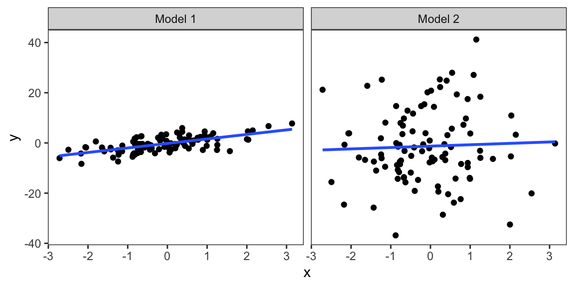
Suppose we have the following two linear regression models fitted to two separate datasets. Which model (model 1 or model 2) do you think exhibits a higher \(R^2\) value?
- Show that the \(R^2\) value for a prediction model is equal to
\[1 - \frac{\text{(RMSE of Prediction Model)}^2}{\text{(RMSE of constant mean model)}^2}\]
- In Table 7.6 in the Housing Tax Assessment case study, we see that after adjusting for the bedroom count and the lot size, one extra bathroom is associated with an increase in the assessed value of the house. However, from the same table, we can see that if you adjust for the bathroom count and the lot size, an extra bedroom is associated with a decrease in the assessed value. How would you explain this negative association for an extra bedroom after adjusting for bathrooms and lot size?