2 Knowing Your Dataset

Background

In the previous chapter, we introduced the data-generating process and the data collection process. Sometimes you might be in charge of the data collection process, and sometimes you might be downstream of it, using a dataset collected by others. In the latter case, you will need to spend some time learning what the data in a dataset mean. Thus, this chapter outlines the basic level of understanding that an analyst must have of a dataset in order to start analyzing the data in it.

Let’s begin this chapter by revisiting an example from the previous chapter: you observe someone flipping a coin. In this example, you witness the data collection firsthand, and in turn, develop a clear understanding of the data’s meaning. If you were to look at the resulting dataset and see a column of data called Heads containing the values True and False, you would know that the data were about coin flips. And more specifically, you would know that the value True refers to a coin flip resulting in a heads, while False refers to a coin flip resulting in a tails (assuming a fair coin).

However, suppose you do not observe someone flipping a coin but instead find a dataset titled “Coins.” Like before, it has a column named Heads containing the values True and False. You might reasonably guess that the data are about coin flips, but it would be very important to confirm that this is in fact the case. Because maybe the data are not about coin flips at all. Rather, maybe each row refers to a different type of coin, and the value in the Heads column refers to whether a coin has a head on it somewhere. Alternatively, maybe the dataset is in fact about coin flips. However, now each value in the Heads column corresponds with the result from two coin flips, and the value True refers to a result in which both flips were heads.

For these alternative scenarios, consider the following: What might it mean if this column contained the values 0, 1, and 2 instead of True and False?

Understanding the exact meaning of your data and how the data are recorded within the dataset is a crucial first step in data analysis. If you collected the data yourself or played some role in the data collection process, this step will likely not take a long time, if any time at all. But often data analysis involves the use of some data that you have found or that have been provided to you. In these cases, taking time to understand your data can help to prevent you from doing an analysis that is misguided or from misinterpreting the final result of your analysis.

In the remainder of this chapter, we introduce a series of “checkpoint” questions for knowing your dataset. We then introduce the strategies and vocabulary required to answer these questions thoroughly.

2.1 Checkpoint Questions

The checkpoint questions for knowing your dataset focus on the meaning and format of data. It is important that an analyst can confidently and accurately answer all of the checkpoint questions before they proceed to the next step of the analysis. The answers to these questions represent a basic level of understanding (of one’s dataset) fundamental to the analysis. The checkpoint questions are as follows.

Q1: What is the unit of observation?

Q2: What are the variables?

Then for each variable:

Q2.1: What does the variable refer to?
Q2.2: What is the variable type?
Q2.3: What is the variable implementation?

Q3: How many observations are there?

2.2 Observations and Variables

To answer checkpoint questions Q1 and Q2, an analyst must be able to identify the unit of observation and variables in their dataset, respectively. The unit of observation is who or what the data are about. This could be a person, a specific item, an event, etc. In the coin flipping example, the unit of observation is a coin flip. Meanwhile, a variable is a particular measurement or piece of information about the unit of observation. In the coin flipping example, one variable could be the Type of coin that was flipped. Another variable could be the Result of the coin flip.

An observation, the focus of Q3, refers to the data collected for one realization of the unit of observation. In the coin flipping example, the data for each coin flip are an observation. Suppose a nickel is flipped and the result is a heads. The data for that observation would be nickel and heads.

2.2.1 Tabular Data

Often, you will see the data for observations and variables organized in a two-dimensional table with rows and columns (e.g., see Table 2.1). Data arranged in a table are called tabular data. In this book we focus primarily on tabular data, and in particular, tabular data that are tidy, a specific and widely-used format for tabular data. Each observation is allocated a row in the table. Each variable is allocated a column in the table. And each cell in the table contains a single data value. In the tidy tabular format, there can be only one unit of observation per table but many observations (rows) and variables (columns).

The dimensions for tidy tabular data are reported as two key numbers: the number of observations (rows) and the number of variables (columns). The number of observations is always listed first, followed by the number of variables. You will typically see this written as observations \(\times\) variables. For example, the dataset in Table 2.1 is 4 \(\times\) 2.

Table 2.1: Example dataset about coin flips with four observations and two variables.

Type	Result
nickel	heads
nickel	heads
quarter	tails
dime	heads

Ultimately, arranging and storing data in a tidy tabular format is both efficient and effective. The data points associated with each observation stay linked horizontally, and at the same time, the data points associated with each variable stay linked vertically. Analysts can then access and work with certain observations and variables by accessing specific rows and columns, respectively.

Given this newly introduced data format, let’s revisit our checkpoint questions Q1 (What is the unit of observation?) and Q2 (What are the variables?). Looking at the example dataset in Table 2.1, we can see that the unit of observation is implicit, while the variables are explicit (the column names). This difference is important to keep in mind when answering Q1 and Q2. When looking at a dataset for the first time, the answer to Q1 might be less obvious. Helpful questions to consider when trying to answer Q1 are the following. Who or what does each row, or observation, in the dataset refer to? Who or what are we taking measurements about? In the end, however, it is best to confirm the answer to Q1 by consulting any dataset documentation that has been provided to you as a data user. Dataset documentation is the focus of a later section in this chapter.

Additionally, revisiting Q3 (How many observations are there?), we can now see that for tidy tabular data the answer will simply be the number of rows in the table.

2.3 Variable Types

Now that we have introduced what a variable is, we can introduce the concept of variable types. The variable type largely determines how the data for a variable are treated in subsequent steps of a data analysis. Checkpoint question Q2.2 is about the variable type.

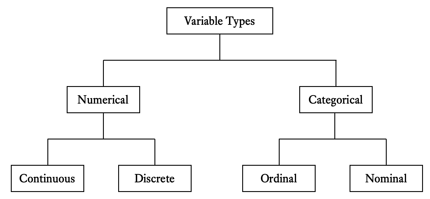
Figure 2.1 is a diagram of different variable types. At the top of the diagram, there are two broad types of variables: numerical and categorical.¹ Numerical variables contain numeric measurements or counts. Categorical variables contain categories or groups. It is important to note that it is not valid to simply say that numerical variables contain numbers, while categorical variables contain categories. This is because it is not uncommon for the categories or groups of a categorical variable to be represented by numbers.

For example, suppose you have a variable called Year, and it refers to the class year of a university student: freshman, sophomore, junior, or senior. In the dataset, this could be represented by the integers 1–4, with 1 representing freshman and 4 representing senior. Although the variable contains numbers, it is still considered categorical because the numbers represent groups.

Now moving to the next level of the diagram, we can see two common types of numerical variables: continuous and discrete. Continuous variables can take on any real number within an interval, while discrete variables cannot. Let’s consider two example variables to explore this difference.

Suppose we have a dataset about classrooms at a university. One variable in the dataset, Temperature, refers to the temperature in degrees Fahrenheit of a classroom at 10 a.m. Another variable, Seats, refers to the number of seats in a classroom. Temperature is continuous, and Seats is discrete. For Temperature we might reasonably expect that most values will fall somewhere between 65–75. And within that range, any real number would be a valid, meaningful measurement. We can measure temperature with varying levels of specificity. The value 65 is interpretable and so is 65.8421. In contrast, we have the variable Seats containing seat counts. This variable does not take on any real number within an interval. A classroom might have 30 or 31 seats, but it cannot have 30.82 seats.

As for categorical variables, there are also two main types: ordinal and nominal. Ordinal variables are those in which the categories or groups have a natural ordering to them. Nominal variables are those in which there is no inherent ordering to the categories or groups. It is also important to note that categorical variables with only two categories (e.g., true/false, pass/fail, low/high, etc.) are commonly referred to as binary variables.

The aforementioned variable Year (referring to class year) is an example of an ordinal variable. Freshman is before sophomore. Sophomore is before junior. Junior is before senior. Alternatively, an example of a nominal variable might be a student’s Major, which could contain values like biology, English, business, psychology, mathematics, etc. Here, there is no inherent ordering to the different categories. If the variable were instead STEM and referred to whether or not a student was a STEM (science, technology, engineering, and mathematics) major, that would be a binary nominal variable.

It should be noted that you may encounter variables that do not fit neatly into the hierarchy shown in Figure 2.1. For instance, a variable containing free form text would not be numerical or categorical. But it may contain important data for the analysis, nonetheless.

2.4 Variable Implementations

In the previous section, we focused on variable types, or what the data for a variable represent. Are the data numerical measurements, categories, or neither? In this section, we focus on variable implementations, or how the data for a variable are represented. Are the data numbers, text, Boolean values, timestamps, etc.? The answer to that question is the answer to checkpoint question Q2.3.

Let’s begin this section by considering the coin flip dataset from before (Table 2.1). It contained the categorical variables Type and Result, which contained words like nickel and heads. In other words, both variables were implemented as text, or sequences of characters (letters, numbers, symbols, spaces, etc.).

In Table 2.2, we reprint the dataset but with two different variable implementations. Now the variables Type and Result are implemented as numbers rather than text. In the Type column, the numbers 1, 2, and 3 stand for nickel, dime, and quarter, respectively. In the Result column, the numbers 1 and 0 stand for heads and tails, respectively. Despite the different implementations, the variables still mean the same thing and remain categorical. Note that using numbers to represent categories is sometimes referred to as coding or encoding.

Table 2.2: Coin flip dataset from Table 2.1 but with different variable implementations.

Type	Result
1	1
1	1
3	0
2	1

So why is knowing the variable implementation important? When we know a variable’s meaning, type, and implementation (i.e, we can answer checkpoint questions Q2.1–Q2.3), we can begin to meaningfully work with the data for that variable.

For instance, when Type and Result are implemented as numbers, we could technically compute the mean of their values. The mean of Type is 1.75, and the mean of Result is 0.75. But does that action—computing the mean—make sense for these variables given what we know about them? For the variable Type, we know that the numbers represent arbitrary encodings for three nominal categories: nickel, dime, and quarter. If we were to compute the mean, we would be finding the “average coin type,” and that does not make much sense. It may make sense though to compute the mode, which would tell us which type of coin was flipped most often. In this case, the mode is 1, or a nickel.

For the variable Result, we know that it is binary (heads or tails) and implemented as 1s and 0s. With this particular implementation of a binary variable, we can compute the mean, and the output is interpretable. Namely, the output is a proportion. In this context specifically, it is the proportion of coin flips resulting in a heads.

In short, it is the combination of meaning, type, and implementation that informs how we work with variables in a data analysis.

2.5 Dataset Documentation

As noted at the beginning of the chapter, if you collected the data yourself or played some role in the data collection process, answering the checkpoint questions will likely not take a long time, if any time at all. However, if you did not have any involvement in the dataset creation, answering the checkpoint questions will require more time and effort. In particular, you will most likely need to consult some form of dataset documentation to learn about the dataset.

The dataset itself is usually limited to 1) the variable names—which may be quite short for practical reasons, such as being easier to reference in computer programming contexts—and 2) the data values. In other words, datasets efficiently arrange and store collected data for use in analyses, but they lack comprehensive description of what the collected data mean as well as how, when, and why they were collected. As a result, an analyst looking at a dataset might be able to guess or infer the meaning of what they see in a dataset but ultimately not know for sure. Dataset documentation is meant to address this gap in understanding, providing crucial information for data users. Dataset documentation is sometimes referred to as metadata, or “data about the data.”

The amount and type of documentation generated for datasets varies. Dataset documentation might cover topics such as the motivation for creating the dataset, the variable definitions, the data collection process, any applied data edits or transformations, the timeline and protocol for data updates, recommended uses, contact information for the dataset creator(s), licensing, etc. When using a dataset downloaded from the web, reading information provided by the dataset creator(s) on the download page is a good place to start. From there, you will likely want to search for a data dictionary and/or a README file.

The name “data dictionary” indicates what the resource provides: definitions. Specifically, data dictionaries provide definitions for the variables in a dataset, making it an especially helpful resource for answering checkpoint questions Q2.1–Q2.3. Meanwhile, the name “README” is an instruction for analysts. Specifically, a README file is meant to be read, as it contains important information for data users to be aware of before using a dataset. README files are commonly located in the data directory alongside the dataset file.

Let’s suppose that—for a dataset—dataset documentation has been provided on the dataset homepage, in the data dictionary, and in the README file, and this documentation has made it easy for you to understand the exact meaning of all the data. This scenario represents a best case scenario. However, sometimes understanding the meaning of your data is neither a straightforward nor quick task and may require substantial reading, thinking, and searching through the documentation. Ultimately, if you cannot figure out the meaning of the data based on the documentation that has been made available to you, it may be necessary to inquire with the dataset creator(s) directly.

2.6 Example: Barton Springs Salamander Dataset

At the beginning of the chapter, we put forward a series of checkpoint questions. These checkpoint questions serve as a basic check for analysts: Do you know the meaning and format of your data well enough to proceed to the next step of the analysis?

In this example, we demonstrate how to answer the checkpoint questions for a dataset found on the City of Austin Open Data Portal. The dataset is titled “Barton Springs Salamander Eliza Closed Population Capture Histories” and was provided to the portal by Austin Watershed Protection, a department within the city government of Austin, Texas. The dataset is about the Barton Springs salamander—an endangered species endemic to Texas—at Eliza Spring in Austin. Data were collected on individual salamanders over 29 survey periods that spanned a total of eight years (October 2014 to August 2022). Table 2.3 shows the first five (of nine) variables for a sample of five rows from the dataset (Austin Watershed Protection 2024).

Table 2.3: The first five (of nine) variables for a sample of five rows from the Barton Springs salamander dataset (Austin Watershed Protection 2024).

id	period	FirstSection	hist	size
57515	Feb 2018	pool	111	10.09
71025	Aug 2018	pool	011	10.18
77874	Aug 2020	stream	100	24.7
80820	May 2021	stream	001	26.8
85705	May 2022	pool	001	18.5

Most of the information needed to answer the checkpoint questions has been provided on the Open Data Portal. Figure 2.2 is an annotated screenshot from a section of the dataset’s page on the portal. This screenshot represents only a portion of the dataset documentation provided on the portal page. The annotations on the screenshot show where to locate the information relevant to each checkpoint question.

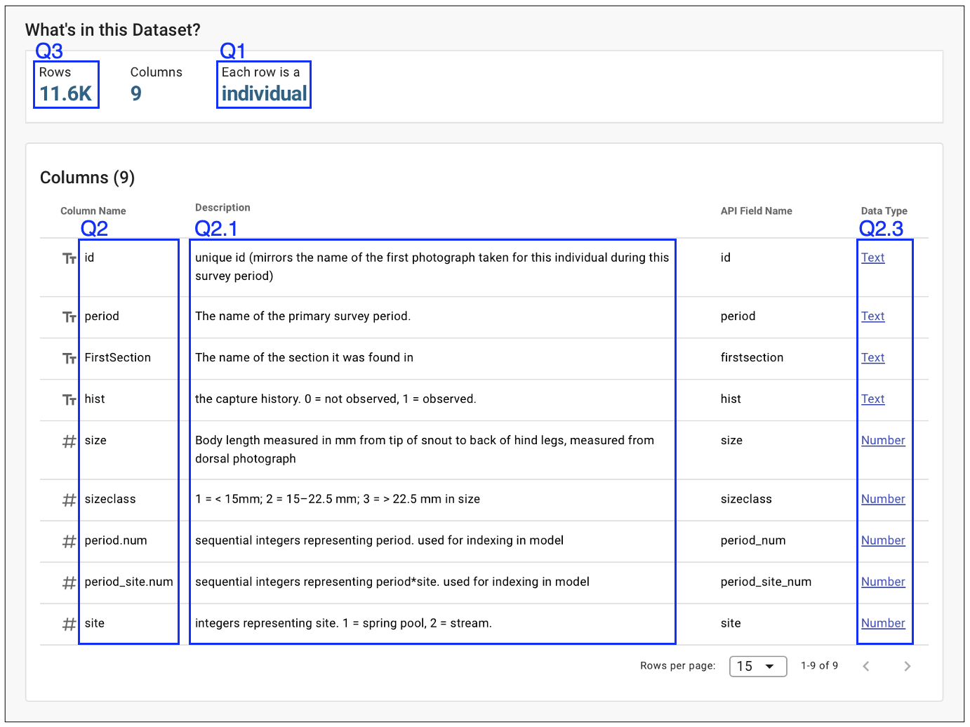
Figure 2.2: Screenshot from the web page for the Barton Springs salamander dataset on the City of Austin Open Data Portal. Blue annotations indicate where to locate checkpoint question answers.

Starting with checkpoint question Q1 (What is the unit of observation?), we can see that the page provides some helpful information. Namely, the page notes that each row refers to an individual. In the context of these data, we can interpret this as meaning an individual salamander. Additionally, upon closer inspection of the data in the full dataset, one can see that some salamander IDs (in the id column) appear more than once, meaning those salamanders were observed during more than one survey period. Therefore, the answer to Q1 is as follows: The unit of observation is an individual salamander during a particular survey period.

The documentation also lists all of the column names, providing the answer to Q2 (What are the variables?): The variables are id, period, FirstSection, hist, size, sizeclass, period.num, period_site.num, and site. Then to the right of the column names, there are column descriptions and listed data types. These provide the answers to Q2.1 (What does the variable refer to?) and Q2.3 (What is the variable implementation?), respectively.

The information for Q2.2 (What is the variable type?) is not provided directly. However, we can derive it using the other information that has been provided to us. Let’s consider the variable hist, which refers to “the capture history,” where “0 = not observed” and “1 = observed.” From Table 2.3 we can see that the hist values take the form of 111, 011, 100, etc. And as noted in the documentation, the variable is implemented as text. Putting these different pieces of information together, we can conclude that each value is a sequence of 0s and 1s indicating how many times a salamander was observed. In other words, the value 111 is not one hundred eleven. Rather, it means the salamander was observed all three times during the February 2018 survey period. Thus, hist is a categorical variable, and in particular, a nominal variable. The different combinations of “not observed” and “observed” have no inherent ordering.

To summarize, the answers to Q2.1–Q2.3 for hist are as follows.

Q2.1: The variable refers to the capture history, where 0 is not observed and 1 is observed.
Q2.2: The variable type is categorical. More specifically, it is nominal.
Q2.3: The variable implementation is text.

The last checkpoint question Q3 (How many observations are there?) can be answered to a degree by looking at the documentation. In the top left corner of Figure 2.2, the number of rows is listed as 11.6K. Upon closer inspection of the dataset, though, we can see that this value is rounded. The exact answer to Q3 is: There are 11,551 observations.

2.7 Summary

When you obtain new data, it may be tempting to jump straight into data exploration and then modeling. However, the outputs of any exploratory tasks or modeling will be meaningless if they cannot be interpreted accurately and precisely.

The ability to accurately and precisely interpret outputs depends not only on a thorough understanding of the analytical methods you are using but also of the data you are using. In this chapter we introduce the process of getting to know your dataset. Specifically, we introduce a series of checkpoint questions about the observations and variables in a dataset. Being able to answer these checkpoint questions confidently and accurately is an important first step in data analysis.

2.8 Exercises

For the Barton Springs salamander dataset discussed in the case study (see Table 2.3 and Figure 2.2), what is the answer to checkpoint question Q2.2 (What is the variable type) for the variables size and sizeclass? How are these two variables related? What would the value of sizeclass be if a salamander was 20 mm in size?
You have been tasked with analyzing housing data. The first three variables in the dataset are residence_type, total_income, and household_size. The survey questions used to collect data for these variables are listed below.

[residence_type] Do you currently rent, own, or have another housing arrangement?

[total_income] What is your household income?

[household_size] How many members are there in your household?

For each variable, list the expected variable type and implementation.

Sketch an example row for the dataset (i.e., a 1 x 3 table). For each variable, include an example value that represents what you would expect to see in the dataset, given the variable types and implementations specified above.
Suppose you see the documentation for some opinion polling data that you are interested in using but that you do not yet have access to. In the documentation, you see that there is a variable in the dataset called age, that refers to the age of each person in the survey. You notice that it is listed as a categorical variable. What format might this variable be in, i.e., what are possible categories for age? Given your answer to the first question, would you classify the categories as ordinal or nominal?

Sometimes the terms quantitative and qualitative are used instead of numerical and categorical, respectively.↩︎